Google offers users a very useful service, called Google Drive. It is a web service, developed in an environment of cloud computing based on software ., which allows you to store and synchronize your documents and files online, including the management of spreadsheets, with the Google Sheets tool.
Google Drive: what it is and what it offers
Google Drive includes services from file hosting, File sharing and collaborative editing of documents and can be used both from desktop and mobile, even through a special app (for Android and iOS). To use Drive from a PC you just need to have any web browser installed, without the need to install any component locally.
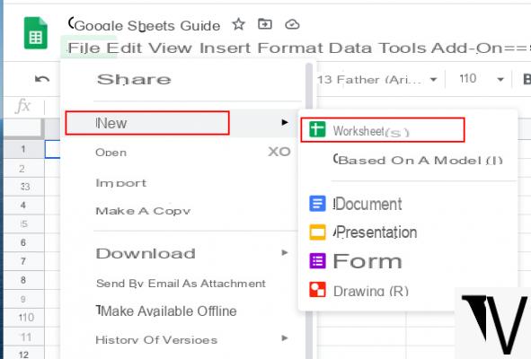
Among the strengths of the tool is that of constantly save on the cloud automatically the work you are doing, allowing you to navigate between the various versions and revisions of the file (possibly indicating the author of the change within reach), to restore those of your interest at any time and to "undo", canceling what was previously typed , practically indefinitely, up to the origins of the file. To access the history of Google Sheets just go to the “File” menu, select the item “Version history”, then “View the history of Google Sheets versions”.
Obviously it is also possible to work on the document offline (when you go back online the work will be synchronized) and share the file with other collaborators, allowing them to modify the file or simply to be able to read it. In order to work offline it is necessary to set the option from the "File" menu, selecting the "Make it available offline".
To share a file you need to go to "File" then on the item "Share"(Alternatively, you can simply click on the button that appears at the top right of the" Share "or" Share "screen), enter the email address of the person with whom you intend to share the spreadsheet and assign the authorization level (such as "View Only" or "Can Edit"). In addition, by going to the “Advanced” menu, you can select any additional privacy conditions.
Within Google Drive we find, in addition to the possibility of storing files in any format on the cloud (the free Drive space available is 15 GB), a suite that is basically proposed as a free and cross-platform alternative to Microsoft Office. It includes tools comparable to Microsoft Word, which in Google Drive is called Google Docs or Google Docs, Microsoft Powepoint, which in Google Drive is called Google Presentations or Google Slides, Microsoft Excel, which is called in Google Drive Google Sheets or Google Spreadsheets, and so on.
Let's see how Big G's alternative to Excel, Google Sheets, works to create gods spreadsheets online, eventually to be exported to your PC, and how to exploit its main features, setting the most common and most useful formulas.
Google Sheets: how to apply formulas
Google Sheets supports the same cell formulas which are normally available in most spreadsheet processing programs. So if you are used to using Microsoft Office or OpenOffice or LibreOffice, etc. you will have no problem using Google Spreadsheets in the same way and taking advantage of being able to work online, even from multiple devices, wherever you are, without losing your work.
Going back to Google Sheets features, these can be used for create formulas that process data and calculate strings and numbers, to generate graphs, but also to highlight cells, to dynamically change the spreadsheet layout, to import data from an external source, to create pivot tables and so on.
The language to be used, according to your habits, for the functions can be changed, choosing between English, Italian and others 21 languages.
enter a formula you have to perform the following steps:
- open a worksheet;
- position yourself in the cell where you want to insert the formula;
- type in the cell the equal symbol (=) followed by the function you want to use.
You can also view suggestions of formulas and intervals based on data: a help window on the function is displayed throughout the modification procedure, indicating the user the definition of the function and its syntax, as well as a useful reference example. If you need more information, just click the “Learn more” link at the bottom of the help window to open the full article.
Google Sheets: how to select data
To quickly select all the contents of a column, simply press the CTRL + SHIFT key combination and move with the down or up arrow. To select a row, instead you have to press CTRL + SHIFT then move with the right or left arrow.
- cell ranges they are indicated with the syntax “A1: B2”, ie by inserting the start and end cells, inserting the colon (:) between them. Comma (,) is used to select non-contiguous cell ranges, for example: (A2, A4, A7).
select an interval of cells to which to apply the formula, indicated by a gray bracket that appears next to the cursor where the range in the formula must be specified, just move with the keyboard arrows on the sheet. Alternatively, you can click inside the sheet to select a range while editing the formula. Of course, you can also select non-adjacent ranges. To select multiple cells, click and hold CTRL on your keyboard (CMD on a Mac) while selecting the cells you want to include in the formula.
An appropriate use of parentheses allows you to use nested formulas. An example of a nested formula: = ABS (SUM (A1: A7)) which calculates the absolute value of the sum. When you select a formula that is inserted into a cell, where other cells are referenced, those cells are highlighted in contrasting colors to help you understand what you are doing more easily and create a formula correctly.
Google Sheets: relative and absolute references
By dragging the formula to a neighboring cell, this will re-elaborate the values to be taken into consideration, adapting in parallel the point to be taken as a reference. For example if you are adding all the values of a range, moving the formula to the beginning of the next column, Sheets will calculate the new sum referring to the new column. In this case we speak of relative references.
But if we don't want this to happen, gods can be used absolute references prefixing the letter indicating the column and / or the number representing the row with the dollar symbol ($). For example, if we want the cell containing the fixed increment value (A1 for example) to be locked both in the column and in the row reference, we will need to insert it in the formulas as an absolute reference, that is, in the syntax $ A $ 1. If the one to keep fixed is only the row reference, but not the column, the symbol must be inserted in mixed mode, for example A $ 1. Same thing if only the column ($ A1) has to be kept fixed.
Google Sheets: how to block the header row
The function of blocking of rows or columns header. The block creates a movable row or column that always remains visible while scrolling, down or to the side, the information contained in the various cells. For example, if you use the first row to label columns, you can freeze that row so you don't have to remember what each column is as you scroll. This is possible by going to the "View" menu and choosing the option "Block"> "1 line" (or up to X lines). Alternatively, you can select the row that appears grayed out a little more often and drag it to the column or row you want to block.
Google Sheets: the main formulas
Once you have entered the data and understood how Google Sheets works, you can process some information using the main formulas that are most often used in this area. So let's see how the basic formulas work that all those who approach spreadsheets, or worksheets, should know:
- SUM. The syntax is: = SUM (range). This formula sums all the values within a selected range;
- MEDIA. The syntax is: = AVERAGE (range). This formula calculates the average of the values within a range;
- FILTER. The syntax is: FILTER (range, condition 1, [condition 2]). This formula returns a filtered version of the source range, returning only rows or columns that meet the specified conditions (a useful application is segmenting data by month and year);
- FIND. The syntax is: FIND (search_for, text_to_search, [starting_at]), the search formula is case sensitive. This formula returns the position where a string is first found in the text;
- COUNTIF. The syntax is: = COUNTIF (range, criterion). This formula returns a conditional count over a range, which is the number of cells that match the proposed criterion. Example: = COUNTIF ($ D $ 1: $ D $ 3253, “Editor”) counts all articles published by the author Editor in the selected range;
- CONCATENA. The syntax is: = CONCATENATE (Value1, “”, Value2). This formula allows you to combine values from multiple cells into one cell, such as First and Last Name;
- NEAR.VERT. The syntax is: = VLOOKUP (search_key, range, index, [is_sorted]). This function is one of the best known in spreadsheets and corresponds to vertical search. Basically what this formula looks for is the first column of a range for a key and it returns the value of a specific cell in the found row;
- SPLIT. The syntax is: = SPLIT (text, delimiter, [split_by_each]). This formula splits the text around a specified character or string and places each fragment in a separate cell in the row. In practice it is the inverse function to CONCATENA and is used for example when you want to divide the first names from the last names in a list of customers or users;
- SUBSTITUTE. The syntax is: = SUBSTITUTE (text_to_search, search_for, replace_with, [occurrence_number]). This formula replaces the existing text with the new text indicated in the string. A very useful function, for example, when you want to replace or update the name of a product or a slogan;
- PROPER. The syntax is: = PROPER (text). This formula capitalizes words with a text string, so you don't need to manually format each entry.
To find out more formulas, at this link you can consult all the formulas supported, or not, by Google Sheets.
Google Sheets: Conditional Formatting
Using the bar at the top, you can format the worksheet to your liking, for example by inserting bold, italics, changing the fonts or colors of the text and cell background. The tool, as well as the other software for managing spreadsheets, allows you to insert formulas for the conditional formatting, to be automatically applied to the selected cells when the condition set in the formula occurs. For example, you can choose to highlight a cell in red if the entered value is less than a certain threshold, or if there are particular strings inside, for example "Error". Or again, it is possible to count the occurrences of a certain type, for example how many cells are not empty or contain a certain term.
Google Sheets: the relationship between Tab
Several can be created within a single spreadsheet Tab thematic in order to organize data and information in a more orderly and elegant way. The data present in the various Tabs can also be recalled in the other tabs, with simple functions. Let's assume we have created a Tab for each month of the year and want to summarize the main results obtained in a summary Tab. In this situation, as in other similar ones, this feature is very useful.
The syntax is = SheetName! Cell. All the formulas described above and all those available in Google Sheets can be applied to it.
Google Sheets: how to import data from web pages
Google Sheets allows you to easily import data from a web page that you are consulting, if the data has been structured in the form of a table. Just select the table in question and then paste it into the application. Sheets will manage everything automatically, inserting the data correctly and making it ready to be modified.
Can also use the function IMPORTXML which allows you to extract data from any web page by automatically dividing them into cells based on the HTML tags within which they are enclosed.
Google Sheets: how to export in .xls and .xlsx format
With Google Sheets you can import and export data in the most common formats (including .XSL, .XSLX, .ODT, .PDF) so that the spreadsheets can be freely reused by users and the data is not tied to a specific platform. To import an Excel spreadsheet into Google Sheets just go to "File", select "Import", then "Upload" and select the file in one of the non-password protected formats. To export the file you need to follow the path "File", "Download" and choose the format in which you want to save the file locally.
Google Sheets: Guide to the main functions