Microsoft Excel has been present on your computer for some time and, looking at its icon, you have well thought of starting to take full advantage of it to help you with everyday operations. Among the many possibilities, you have decided to use worksheets to keep track of your university performance, so that you always have the statistics on the progress of your studies at hand.
Once you created the spreadsheet though, you realized you didn't have a clue of how to average on excel and you are afraid of having to perform arithmetic operations with the classic calculator, and then manually update the recorded values: don't worry, it's not like that at all! There are, in fact, functions that allow you to calculate the mean, the mode and the median and to automatically update the values without performing complex manual calculations: below I am going to explain how each of them works.
So what are you waiting for? Read carefully all the instructions that I am going to give you, put them into practice and you will see that, at the end of this guide, you will use the Excel formulas relating to the calculation of average values as if you were an expert user! Before taking action, however, I would like to make you a small clarification: in the guide below I will make use of Office 2022 for computer (compatible with Windows and macOS). However, you can also apply the same procedures on Excel Online and Excel apps for Android and iPhone / iPad.
Index
- How to do the arithmetic mean in Excel
- How to do the weighted average in Excel
- How to average your marks in Excel
- How to calculate the median in Excel
- How to calculate fashion in Excel
How to do the arithmetic mean in Excel
La arithmetic average, Or simply media, in its simplest definition, it is nothing more than the intermediate value that lies between the upper and lower extremes of a series of values. Speaking in practical terms, the average is the sum of the values included in a set divided by the number of the values themselves: if, for example, we consider a set composed of the numbers 1, 5, 11 and 27, the arithmetic mean is given by the formula = (1 + 5 + 11 + 27) / 4, i.e. 11.
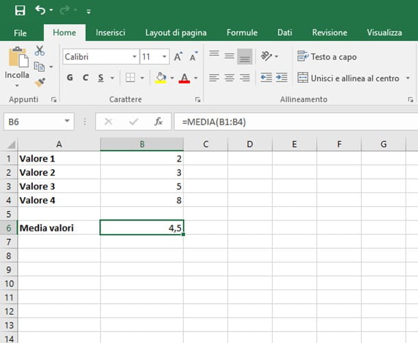
Microsoft Excel has a pre-set arithmetic operator called MEDIA, which allows you to quickly calculate this value by defining a range of rows and columns: all you have to do, in practice, is to define the set of cells to calculate the average of and specify it in Excel. So let's see a practical example on how to do the arithmetic mean in Excel.
If, for example, you want to know how to calculate average age in excel, whose values are contained in the cells B1, B2, B3 e B4, you must specify to the operator MEDIA the parameters B1: B4, that is, the name of the first and last cell involved in the calculation. To proceed, click on the cell in which you want to store the average (e.g. cell A13) and enter the formula = AVERAGE (B1: B4), and then press the key Submit of the keyboard.
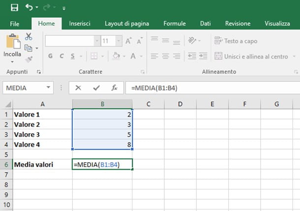
Alternatively, after clicking on the empty cell, click on the symbol ƒ? located in the toolbar immediately above the work grid (on the left), click on the item MEDIA attached to the panel that opens immediately after, press the button OK, enter in the field Num1 the text B1: B4 and click on the button OK.
If you want to know how to average values in excel which are in different cells, therefore not belonging to the same row or column, you must perform this operation: you must specify the aforementioned cells between the brackets of the operator MEDIA, separating one from the other with a ; (semicolon). For example, if you intend to calculate the average of the cells A5, B9 e C4, you must specify in the cell that will contain the result the operation = AVERAGE (A5; B9; C4).
If you want to do the average on Excel excluding zeros or excluding empty cells (for Excel a blank cell equals zero), you need to use the function instead MEDIA.SE(). The operation is very similar to what we saw with the operator illustrated in the previous lines: in the formula = AVERAGEIF (B1: B4; "0") you must define the range of values on which to calculate the average (B1: B4) and then set the policy "0", to indicate all non-zero values.
Finally, it may be useful to calculate the average in Excel with filter set on the data table. This is useful if you want to see the average vary based on the data displayed via the filter. In this case, you have to use the formula = SUBTOTAL (1; B1: B4), in which the value 1 defines the average to be performed, while B1: B4 the range where all the data is present.
How to do the weighted average in Excel
La weighted average, also known as weighted average, is an indicator of the average value of a set of elements, in which each of them is influenced by a specific weight, which defines its importance. In practice, the weighted average calculation is often used to calculate the average value of assets considering market fluctuations or to calculate the degree grade (in this case, the "weight" is the value in educational credits of the exam itself: I'll tell you more about it in the next section).
Having made this necessary premise, it's time to take action: arithmetically, the weighted average is the sum of the products of each value by the respective weight, all divided by the sum of the weights. In practice, there is no specific function for make the weighted average on Excel, but you need to combine the three operators that I show you below.
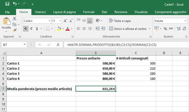
- SUMPRODUCT () - it is an operator that multiplies each cell with its weight and returns the sum of the calculated values. For example, assuming the value of an item is specified in the cells B2, B3, B4 e B5 and the respective weights in the cells C2, C3, C4 e C5, the operator syntax is = SUMPRODUCT (B2: B5; C2: C5).
- SUM() - is the operator that allows you to add the values of a set of cells. Thus supposing that we need to add together the weights of the elements, contained in the cells from C2 a C5, the syntax = SUM (C2: C5) must be used. You can find more information about this operator in my guide on how to sum in Excel.
- / - it “slash”, inserted within a formula, denotes the division operation between two elements.
So, to calculate the weighted average on the values in cells B2 to B5, with weights specified in cells C2 to C5, click on the cell that must contain the result (e.g. B8), write in it = SUM .PRODUCT (B2: B5; C2: C5) / SUM (C2: C5) and press the key Submit on the PC keyboard: as if by magic, you will see the weighted average value appear in the chosen cell. Remember to adapt the formula to the cells you need to operate on, within your spreadsheet.
How to average your marks in Excel
Now that you've learned how to calculate both arithmetic and weighted average, it's time to teach yourself how to do the grade point average in Excel using a simple worksheet, adapted to two different scenarios: the first concerns the calculation of the "simple" average of the marks, suitable for example for the scholastic judgment, while the second concerns the weighted average of the marks in relation to university credits, very useful to get an idea of the starting degree grade.
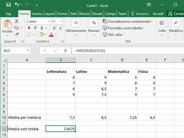
Regarding the calculation of the grade point average, fill in the cells in row 1 of your worksheet (B1, C1, D1, etc.) with the names of the subjects and fill in the respective columns with the marks received in the questions: for example, the cells B3, B4, B5 e B6 contain the votes received in literature, the cells C3, C4, C5 e C6 those received in Latin and so on.
At this point, click on the cell that must contain the average of the marks relating to a specific subject, for example literature (cells from C3 to C6) and type in it the formula = AVERAGE (C3: C6) followed by pressing the key Submit on the keyboard, then repeat the operation for all the other subjects.
If you want, you can do the total average of grades: if, for example, you have entered the average grade for each subject in cells B10, C10, D10 and E10, to obtain the total average, all you have to do is calculate the arithmetic mean of the respective values. To do this, click on the cell in which you want to carry out the operation and type in it the formula = AVERAGE (B10; C10; D10; E10), or =MEDIA (B10: E10), followed by pressing the key Submit.
As regards, however, the weighted average of the marks, that is the one useful to relate the exams with the university formative credits, you can act in the following way: fill in the column A with the names of your exams, enter in the column B their respective votes and in column C the training credits assigned for each exam.
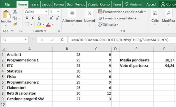
Assuming that the exams to be taken into account are 9, therefore 9 rows in total, choose the cell in which to calculate the weighted average (eg. F2), enter the operation = SUMPRODUCT (B1: B9; C1: C9) / SUM (C1: C9) and press the key Submit on the PC keyboard.
At this point, considering that the starting degree grade is given by the product of weighted average by 100, all divided by 30, choose the cell in which to calculate the starting grade, type in it the formula = (F2 * 100) / 30 and then press the key Submit. For more clarification on the multiplication operation, I refer you to my guide on how to multiply in Excel.
How to calculate the median in Excel
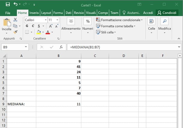
Arithmetically, the median within a series of values it is the one which, once the set has been ordered in ascending or descending order, occupies the central place. If the number of values were even, the "central" ones would be two: in this case, the median corresponds to the arithmetic mean of the aforementioned elements.
Fortunately, in an Excel worksheet, you don't have to manually perform the sorting operations and the subsequent calculation, but you can use the operator MEDIAN() which takes care of doing the work for you: exactly as seen above, you need to specify the cells or the set of cells that contain the values to be calculated.
In practice, to calculate the median of the values entered from cell A1 to cell A10, all you have to do is click in the cell in which to perform the calculation and type in it the formula = MEDIAN (A1: 10) followed by pressing the key Submit. It wasn't difficult at all, was it?
How to calculate fashion in Excel
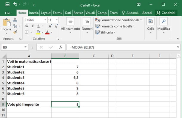
As you may have learned from math or statistics lessons, the fashion, within a set of values, is the one that occurs most frequently, provided it exists.
Just to give you an example, considering the grades of a class in a given subject, the fashion it is that vote that appears most often. The fashion calculation in Excel is simple and is done through the operator FASHION(): inside it, exactly as seen previously, the cells (or cell ranges) from which to extrapolate the mode must be specified.
Therefore, to calculate the mode between the values contained in the cells A1, A2, A3, A4 and so on up to A10, you have to write = FASHION (A1: A10) inside the cell you intend to use to perform the operation. If you need to do this calculation for a very large range of values and you need more precision, you can use the operator FASHION.SNGL in an almost identical way to what has been explained above.
If you have made it this far, it means that you have learned to fully master the calculation of the average through the functions integrated in the program: I bet you now want to know more about the features offered by the powerful program from Microsoft, as you intend to use it for other purposes as well. Well, I think I have what you need! Consult without hesitation my guides on how to make a table in Excel, how to make an invoice, how to add up the hours and how to sort texts in alphabetical order: I'm sure you won't regret it.