You need to create a Excel very well organized, in which you can interact with the items in the cells, through the appropriate lists and drop-down menus? Well, it looks like you need Excel's list functionality. What is it about? Just what I mentioned, that is a function that allows you to group certain cells in separate lists and to create drop-down menus with the items and values present in the spreadsheet.
If you want to know more, take five minutes of free time and find out how to make drop down menus in excel, following the directions I am about to give you. I assure you that this is a very simple operation to complete, you don't need to be an Excel expert to do it.
I bet you can't wait to start reading all the steps to take to reach your goal, right? So let's not waste any more time and let's get to work immediately: you just have to sit comfortably in front of your PC and pay attention to all the operations that I will describe to you. Please note that the procedures are applicable to Excel for Windows, macOS and Excel Online, but not to the Excel app for smartphones and tablets. Having said that, I just have to wish you a good reading and good work!
Index
- How to create a drop-down menu in an Excel cell
- Come fare a cast with Excel
- How to create a dynamic drop down menu in Excel
How to make drop-down menus with Excel
I Excel drop-down menu they can contain values defined directly by the user (therefore words, phrases or figures present exclusively in the menus) or they can be created starting from values already present in the spreadsheet. But let's go in order.
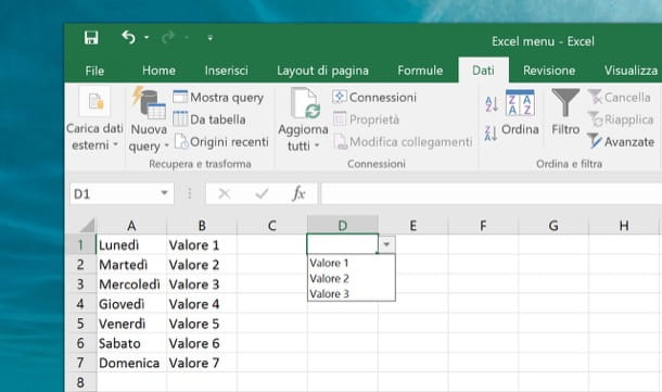
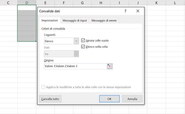
To create a drop-down menu using values defined directly by you, select the cell (or cells) in which to insert the menu, go to the tab Data of Excel, which you find at the top, and click on the button Data validation.
In the screen that opens, select the item List from the menu Allow and type, in the text field Origin, all the values you want to appear in the drop-down menu, separating them with a semicolon. Finally, click the button OK And that's it.
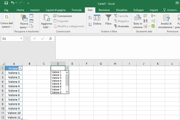
At this point, select one of the cells in which you have inserted your drop-down menu and click on the icon ▼, located alongside. If you have followed the operations I have indicated to the letter, you will be shown a box, through which you can select one of the values you have defined. Convenient, right?
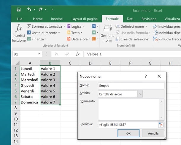
If, on the other hand, your intent is to make a drop-down menu with Excel using the values already present in the spreadsheet, the operation to be performed is similar to that described above. First of all, select with the mouse the cells that contain the values to be inserted in the drop-down menu (the values must be contained in the same column or in the same row and there must be no interruptions between them), go to the tab Formulas of Excel that you find at the top and click on the button Define name.
In the screen that is shown to you, type the name you want to assign to the selected group of values, without inserting any space, and then click on the button OK, in order to save the changes.
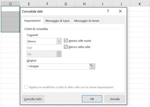
At this point, select the cell (or cells) in which you want to insert your drop-down menu, go to the tab Data at the top, and click the button Data validation.
In the new screen you see, select the item List, using the menu Allow, and then type, in the field Origin, the symbol =, followed by the group name of data you created earlier (eg if you called the group of values "group" you have to type = group). At this point, all you have to do is press the button OK, to confirm the operations you have carried out.
Very well! You have just created a new drop-down menu starting from the values already present on the spreadsheet! To view them, select one of the cells in which you have entered your drop-down menu and click on the icon ▼ opposite: in this way you can choose one of the values from the box that will be shown to you.
Another important thing to know is that the values in the drop-down menu will update in real time. This means that if you change any of the values from the list of the spreadsheet in which you created the drop-down menu, the changes will automatically be made in the menu as well.
Come fare a cast with Excel
Now let's see how to create a drop-down menu to filter and organize the values present in the spreadsheet.
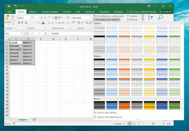
If you want to learn eat fare a cast with Excel, all you have to do is open the document in which you want to insert your lists, click on the button Format as a table contained in the card Home of Excel, at the top, and choose the style you prefer from the menu you see.
At this point, hold down the left mouse button, select all the cells you want to include in your list and click on the button OK, to confirm. If you also highlighted the column titles, put the check mark next to the item Table with headers.
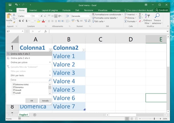
Done! You have just obtained a list where you can organize the values of the cells through special drop-down menus. Indeed, by clicking on the icons ▼ placed on the cells relative to the column headers, you can arrange the values in alphabetical order, apply of filters based on customized parameters, activate or deactivate the display of certain values and much more.
If you want, you can change the style of your table by selecting one of the cells that are part of it and choosing the desired style from the menu Home> Format as a table.
Finally, if you want to cancel the creation of the table, you can click on the button Cancel Excel (theleft pointing arrow icon, which you find right at the top left, in the title bar of the program), or you can select all the cells that are part of it, go to the Planningat the top and click the button Convert to range.
I warn you that you can also get the same result using the function filters Excel: select the column header cell, reach the tab Home and click on the items Sort and Filter> Filter, to activate the drop-down menu.
How to create a dynamic drop down menu in Excel
If you want create a dynamic drop-down menu in Excel, I warn you that this operation is not difficult, but you must be patient and pay the utmost attention to the procedures that I will describe to you.
Actually, if you have already mastered the operations I described to you in the previous chapters, you should be able to easily create this type of menu, as it is the combination of the two methods previously described.
The first thing you need to do is highlight all the cells containing the values you want to enter in the drop down menu. A dynamic menu is created starting from the data already present in the spreadsheet and you cannot, therefore, define them directly, except by inserting them in appropriate cells.
After highlighting the cells, go to the tab Homeat the top and click the button Format as a table, choosing a style from those listed. If you have also selected the column label, check the box Table with headers and then press on OK, to confirm.
Now, highlight the cells of the newly created table, not including thecolumn label (it is generated automatically if it was not already present) and reach the tab Formulas. Once this is done, press the button Define name and indicates a name to assign to the group of values by typing it in the field Full name. Then press OK to confirm this operation as well.
At this point, select one or more cells on which you want to insert the drop-down menu and reach the tab Data. Now, press the button Data validation and, in the screen that is shown to you, choose the item List from the menu Allow. Then type the symbol = followed by group name that you have previously defined. Again, confirm the changes made by using the key OK.
Good! If you have carefully followed the procedures I have indicated, by clicking on one of the cells on which the drop-down menu is present, you will find the icon ▼ opposite: interacting on the latter, you will be shown a box containing values to select, which will correspond to those of the table you have created.
The peculiarity of this menu is that it can add values without having to change any configuration parameters. Simply go to the table, move to the last blank row and add a new value. By doing so, the latter will also be available in the drop-down menu.