 PixieMe / Shutterstock.com
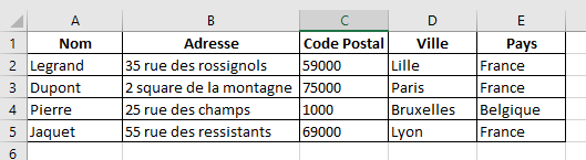
The Excel function VLOOKUP searches for a value in the first column of a table and then returns the value of a cell that is on the same row as the value sought.
Imagine that we have to display Mr. Pierre's country of residence in a cell. The VLOOKUP function will allow us to perform this process very easily.
1. Use VLOOKUP Function Syntax
The standard syntax for this function is: =VLOOKUP(lookup; array; column; type)- In “search”, enter the value to search for in the first column of the table (here, the character string “Pierre”)
- In "table", enter the range of cells that contains the table data (here, A2:E5)
- In "column", enter the column number of the table that contains the result to be returned (here, column 5 for the country)
- In "type", enter FALSE to find the exact value of "search" (if in doubt, enter FALSE to avoid surprises). You can also choose to search for the closest value to "search" by entering TRUE (or leaving it blank).
We apply the following formula in the cell to display the result:
=VLOOKUP("Peter",A2:E5,FALSE)
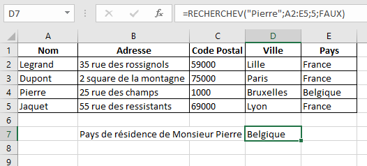
The VLOOKUP Function displays the result "Belgium" in cell D7.
40 ">This tutorial is brought to you by the trainer Jean-Philippe Parein
Find his course Learn and master Excel from A to Z
in full on Udemy.


![[Review] Samsung Powerbot VR7000: the robot vacuum cleaner from Star Wars](/images/posts/6bc44de38605b5c0fa12661febb1f8af-0.jpg)