▷How to use Excel 🥇

Admit it: you and the PC still don't get along very well but, despite this, in the office you were asked to make some spreadsheets in Excel. The challenge is difficult, your knowledge of Office is still quite limited but I'm sure that, with a bit of commitment, you will be able to impress all your colleagues.

No kidding! A few basic notions are enough and using Excel becomes easy and intuitive for everyone. How about if I start giving you some "tips" on how to use Excel and from here do you try to learn all the steps necessary to complete your work? Do you want? Perfect, then sit down comfortably in front of the computer and just dedicate some free time to me, so that you can carefully read all the tips I have prepared for you in this guide of mine.

Just a small clarification before starting: for the tutorial I used the 2022 version of Excel for Windows and macOS but the indications in the guide should also be valid for older versions of the software (and, probably, for future ones too) . Clear? Very well, then I just have to wish you good reading and good work!

Using Excel on a computer

Microsoft Excel is a software that allows you to perform calculations on data, distributing them on tables and graphs. It is a software belonging to the category productivity widely used by both companies and normal users. In fact, it can generally be used to perform even simple home accounting calculations. It is paid and requires the purchase of a user license with prices starting from € 69,00 / year, but a free trial version lasting 30 days is also available and there are online and mobile versions. usable at no cost.

If you have also decided to use Microsoft Excel, download the software following my guide on how to download Excel, then come back here and read the tips you find in this guide. Today, in fact, I will address the Excel topic by illustrating all the main functions and features of this powerful program which, as already mentioned, is available both for Windows that for MacOS, as well as for mobile devices and in the online version.

Create a spreadsheet

The first step to take is to start Microsoft Excel through its icon on the Windows desktop, in the Start menu or, in the case of macOS, in the Launchpad. As soon as the program is opened, you are asked to indicate the model to be selected for data entry.

You can, for example, choose the model Academic calendar, to create an electronic diary, or Employee absence planning, to manage the days of vacation and sickness of its employees.

In our case, however, I'll take care of explaining how Excel works, taking into consideration a blank template. Then select the item Blank workbook to access the Microsoft Excel spreadsheet.

What will be presented to you will be a spreadsheet divided into column e lines, therefore composed of celle. The columns are identified with the letters of the alphabet, while the rows by a progressive numbering. In the upper bar, however, there are some cards that allow you to access all the functions offered by Excel.

In the next few paragraphs, I'll explain how to use some of the most important features available within these tabs. Therefore pay the utmost attention to better understand how the software works.

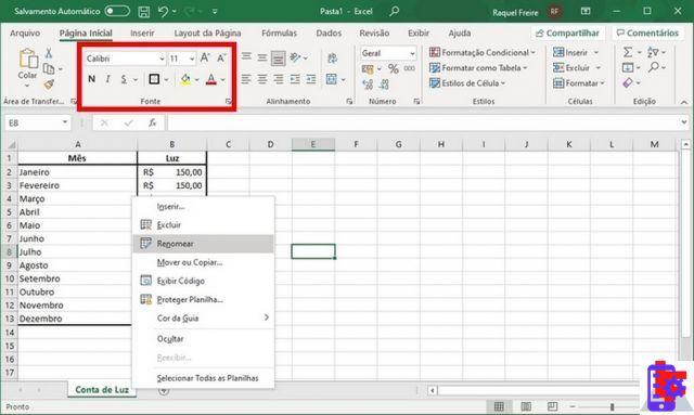
Cell formatting

The Excel spreadsheet is made up of several cells. By double clicking on one of these, you will enter the mode Modification, which allows you to type any type of data or formula. Just as it is possible to do using Microsoft Word, Excel is also possible format the text in order to perform a layout of the data in an attractive and, above all, organized way, in the event that the work is to be presented to other people.

Reaching the board Home, you can find several buttons divided by category that allow you to perform this operation. For example, in the section Character, you can select the font font size, the style (Bold [G], italics [C] and underlined [S]) and the coloration. In the section AlignmentInstead, you can align text left, right and centered or create paragraph indents.

In the Numeri, you can set the way in which Excel should behave when entering data in a cell: by clicking on the drop-down menu with the wording General, you can select the style of the entered data, such as a date, a currency or of the text, just to give some examples.

Also, you can change the size of the columns and lines or insert or delete new ones, using the functions you find in the section Rooms. You can also set gods filters, in case you have arranged the data on a table, using the function Sort and filter, present in the section Modification. In this case, by applying filters on the cells that contain the column labels, you will be able to filter the data using the icon with the symbol (▼).

If, on the other hand, you need to do some quick calculations, in the tab Modification, refer to the function SUM, which allows you to perform the algebraic sum of values present in a user-defined range. By clicking on the icon with the symbol (▼), located next to this function, you can select other calculation parameters, such as media and count of values.

To learn more about how Excel works with regards to basic calculations, I recommend that you consult my tutorials on how to add in Excel, how to subtract with Excel, how to multiply in Excel and how to calculate the percentage in Excel.

Insert pivot tables and charts

Another useful Excel function is the one you need to make table pivot; these allow to summarize the data in a summarized and organized way, according to the parameters established by the user.

To create a pivot table, click on the tab Inserisci and then click on the button Pivot table. Subsequently, you will be able to see on the screen a window requesting the insertion of data from an existing range and the cell where Excel will generate the pivot table. After confirming the requested information, the right sidebar will show you the types of data to drag into the fields filters, Columns, Lines o Values.

If you need more information on how to use a pivot table, I suggest you read my guide dedicated to this topic.

Also, always inside the card Inserisci, you have the possibility to distribute the data on gods graphics. You can, in fact, make histograms, of the graphs in lines, a dispersion o a cake. In short, you have all the types of graphs available to organize your work data.

The specific buttons for each type of graph are present in the section Graphs or you can see them by clicking the button Recommended charts and then selecting the tab All charts, in the screen that is shown. If you want more information on how to create a chart in Microsoft Excel, I suggest you read my guide dedicated to this topic.

Inserting formulas

Another very important functionality of Excel is that related to the use of functions. These are formulas that allow you to perform calculations or to extract information on user-defined intervals.

There are many functions in Excel and these are divided by category, based on their scope of use. Just to give some examples, there are functions belonging to categories Financial, Stats, Logics o Mathematics.

Inserting a function is very simple: to do this, select a cell by clicking on it and then press the key Insert function, which you find in the card Formulas, at the section Function library. At this point, in the next screen that is shown to you, look for the function that best suits your needs.

For example, if you want to capitalize the text of a cell, move to the adjacent one and enter the function SHIFT (...) through the procedure that I have indicated to you in the previous lines. In the arguments screen for the function, you will then be prompted to select the cell to convert to uppercase; after selecting it, press on OK to immediately see the result of the function just inserted.

Data management

In Microsoft Excel it is possible import the data also from external sources: in the card Data, there are some features that allow you to perform this operation.

To do this, click on the button Upload external data: in this way a drop-down menu is shown through which you must indicate the source to use to import your data. You can choose, for example, to import a Microsoft Access database or even a text file.

It may happen that when importing files in CSV, these appear in a single column, rather than spread across a table. How to solve? Simply by clicking on the button Text in columns, present in the card Data and at the section Data tools; this allows you to convert a CSV dataset into an Excel table.

Also, you can apply the data validation inserted in the cells, if these meet the requirements set by the user. To do this, always using the card Data, award-winning Data validation (it is located in the section Data tools).

In this way, a window is displayed that allows you to select the type of data that are allowed at the time of insertion in specific cells. Just as an example, you can choose to only allow numbers within a defined range or to only accept data in date format.

Optionally, you can also set gods input and error messages which are shown to anyone entering data into the Excel worksheet.

File review and protection

Microsoft Excel also includes the spell check, to verify the correctness of the texts in the worksheet. To use it, go to the tab revision and, in correspondence with the section Correction tools, start the Check spellingby pressing the button of the same name.

If you wish, you can also do the translation of texts present in specific cells by pressing the button TranslateIn section Language. Also, if the document is used by multiple people, you can enter comments for the review of the job: all the buttons used for this purpose are present in the section Post comments .

If, on the other hand, you want your work not to be modified by those to whom you distribute the file, you can decide to set one password protection. The buttons Protect sheet e Protect Workbook allow you to perform this operation, blocking the modification of the entire file. Useful, don't you think?

In case you need to make sure that only some cells can be edited, right click on a cell and press on the entry Formato that, in the context menu that is shown to you. In the screen that opens, select the tab Protection, uncheck the box Blocked and then press then OK.

In a nutshell, by acting in this way, if you enable protection on the worksheet as I indicated earlier, the modification will be allowed only for those cells to which the label has been removed Blocked.

Changing the data display and Macros

The display screen of the Excel spreadsheet can be changed using the buttons in the section Immagine. In this section, you can change the visual style, so that, for example, the page breaks or the ruler.

You can also decide to freeze rows or columns so that they always appear when scrolling through a long table. This feature can be activated by clicking on the tab Immagine and then on the button Freeze PanesIn section Window.

Microsoft Excel also allows you to create macro means Microsoft Visual Basic, an advanced programming tool. The latter are nothing more than instructions that are programmed by the user and are useful for carrying out repetitive steps. An example is to create a macro to format the style of the new data entered, according to some precise instructions indicated by the user.

If macros consist of operations to be performed on functions present in the Microsoft Excel interface, just use the button Record macros. Then, in the window that is shown to you, enter the name of the macro, the hotkey and then press on OK to start recording. You must then manually perform the operation you want to automate and then press the button Stop recording, to save her.

With more advanced knowledge of Microsoft Visual Basic, even more complex and elaborate operations can be performed, thus creating an extended level of customization of the spreadsheet.

Save a spreadsheet and print

Have you finished working with the Excel spreadsheet? Very well; at this point you must proceed with the rescue of the file. Basically, Microsoft Excel automatically saves the file every 10 minutes, but you can save it manually by pressing the icon with the symbol of a diskette, which you find located in the upper left corner.

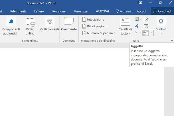
If you want to save the spreadsheet to a specific folder or in another format, click the tab Fillet and then press on the menu item Save with name, located in the left sidebar. Then select the button Shop by Department and browse the computer folders, in order to select the destination where to store the file.

At this point, using the drop-down menu corresponding to the item Save eat, you can optionally choose to save the workbook in another format than the default xLSX. Just to give you some examples, you can use the old format xls or that ods o csv. You can also use Microsoft's PDF printer to save the file in PDF.

If you want, instead, print an Excel file, click on the tab Fillet and then press on the item Print, in the left sidebar. Then choose the printer and configure the settings for printing according to your needs, using the information you see on the screen. At this point, press the button Print to start printing the Excel file.

More useful information on how to use Excel

In addition to the information reported in this guide, you may be interested in some tutorials I made on Microsoft Excel, such as how to use Excel for invoices or how to normalize data in Excel. If you are also interested in reading other tutorials on Microsoft Excel, then I suggest you click this link in order to see all the guides I have written regarding this software.

Furthermore, if you need to study some aspects of this software in particular, I can recommend some books that will surely help you for a professional use.

See offer on Amazon See offer on Amazon See offer on Amazon

Using Excel online

As mentioned above, Microsoft Excel is paid software. For this reason, in case you do not want to buy it, but still want to use its features, I recommend that you consider using Microsoft ExcelOnline.

This tool allows you to work on Excel spreadsheets via browser, just as if you were using computer software. The advantage that can be obtained is that of being able to share documents, so that several users can possibly work on the same file at the same time, if this possibility has been correctly configured.

In this regard, to share a Microsoft Excel Online spreadsheet, click on the button Share that you find at the top right and type the recipient's email address. Then click on the wording Recipients authorized to modify to change the editing permissions of the document and to allow access even to those who do not have a Microsoft account.

Microsoft Excel Online is nearly identical in its functionality to desktop software. Some features, however, are not present in this version, such as the protection of a spreadsheet via password ordata import from an external source. Also, saving files in formats only xLSX e ods.

That said, for everything concerning the functioning of Microsoft Excel Online, refer to the previous chapters dedicated to Windows and macOS, as it is possible to use them in the same way.

Use Excel on smartphones and tablets

If you are out of the office or away from home and don't have a laptop with you, you can rely on the app Microsoft Excel for Android (also on alternative stores) and iOS / iPadOS, so you can work on an Excel file, acting as a smartphone or tablet. The app is free for all devices with dimensions equal to or smaller than 10.1 ″.

Compared to desktop software and online tool, the mobile app has significantly less functionality. Speaking of those present, however, there is the possibility to insert any function in a cell, using the relative button in the upper left corner of the screen, or to change the formatting of the data and the individual cells.

In addition, there are calculation functions, such as the algebraic sum, the average and the count of values, or those for sorting and filtering the data of a table. You can also add tables and graphs or draw freehand.

However, by purchasing the Premium, Available at Microsoft 365, you get access to some additional features, such as the ability to apply multiple colors for formatting or the one you need to change the styles and layouts of pivot tables, for example.

If you are interested in how the app works Microsoft Excel on smartphones and tablets, I suggest you read some of my guides dedicated to the topic: how to use Excel on Android, how to use Excel on iPhone and how to use Excel on iPad.

Use excel without a mouse

You need to know that no matter what device you are using to run Excel, you can use the keyboard to perform quick operations.

For example on Microsoft Excel ed Excel Online, you can use the keyboard instead of the mouse to perform some procedures; on the app Excelon the other hand, by connecting a keyboard, you can avoid making touches on the screen for some operations.

For example on Microsoft Excel for Windowsby pressing the key TAB you can move between the menu tabs at the top by pressing CTRL + Jinstead, you can enter the current time in a cell.

In fact, there are tons of keyboard shortcuts for Excel. If you want to discover them all, both as regards the desktop software, the online platform and the mobile app, I recommend that you view the official Microsoft guide.