You have been asked to make some graphs to represent some data in Excel. The problem is that, among the many graphics available in the famous Microsoft software, you have no idea which one would be the most suitable for the situation. On your spreadsheet you have a data set spread over at least two columns; the first contains labels (or categories) while the adjacent columns contain the data corresponding to each label. If you are faced with this kind of table, your best bet is probably to use a line graph.
You must know, in fact, that a line chart presents the categories of data on the horizontal axis, while the data are distributed on the vertical axis, which are represented with a line. Well: now that you have the final project clear in your mind, it's time to think about how to make it happen. Don't know how to do it? In this case, you don't have to worry, because I'm here to help you.
In fact, in today's guide, I'll show you how to make a line chart in excel, both through the classic Excel for Windows and macOS computers, and on the free Excel Online platform. Also, if you are away from home and need to perform this operation via smartphone or tablet, I will explain how to operate via the Microsoft Excel app for Android, iOS and Windows 10 Mobile. Are you curious to learn more about the topic? Good! Let's not waste any more time and start immediately: sit comfortably and pay attention to the procedures that I will show you in the next chapters. I just have to wish you a good reading and, above all, a good job!
Index
- Make a line chart in Excel
- Make a line chart in Excel Online
- Make a line chart on smartphones and tablets
Make a line chart in Excel
If you want Make a graph to line your Excel, in the next chapters I will show you how to do this in a simple way, which will not take long. In this regard, I advise you to pay close attention to the procedures that I will indicate to you, so as not to make mistakes and, therefore, to create a line chart on your spreadsheet.
Create a new chart
Before starting with the creation of the line chart, it is necessary to make sure that the data is arranged on the sheet in the correct way, as I have already shown you in the previous paragraphs. In the next few lines I'll show you my example, but it can be applied to any dataset.
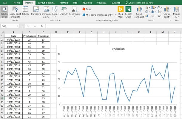
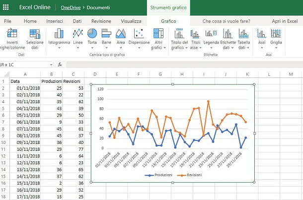
In my example, I have three columns with data: in that A the days of the month are shown in a progressive and increasing manner distributed on the underlying lines; in the columns B e C I have data that correspond to a series of values collected daily, according to the values in column A. You could also have data set according to a chronological order or simply data attributed to categories, such as the quantity of products and the profits made by the different collaborators, just to give you some examples.
Remember to add headings on each column, mirroring the categories of data that are distributed under each of them. In my example, on the column A I'll point to the label Data while, on those B e C, I will indicate Productions e revisions.
For a line chart, you don't necessarily need both columns B and C, but you could only use one of them - in this case, you'll only be representing a single-line data set. Using both columns, however, would have a two-line representation. Let's go in order.
At this point, you need to insert the line chart. Let's start with a one-line chart only: highlight the data contained in the category column (A) and data (B), including labels. Then hold down the left mouse button on the cell containing the label of column A and drag the selection box to the end of the table, that is, to thelast cell of the data in column B. You can also click on the first cell (the one with the label in column A), hold down the key Shift and finally click on thelast cell of the data in column B.
With that done, move to the tab Inserisci and press pulsating Recommended charts, which you find in the section Graphs. In the screen that is shown to you, select the tab All charts and choose the icon Tiers o Lines with indicators. Alternatively, go to the tab Recommended charts and select the chart Tiers, among those proposed to you. Once this is done, click on the button OK to insert the graph into the spreadsheet, which you can drag anywhere.
Enter data into a chart
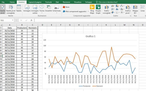
According to what I indicated in the previous chapter, you can also select multiple data sets, so as to create a two or more lines chart. I remind you, however, that on a graph with two or more lines the visualization may not be satisfactory, if the data are not uniform according to the same scale. Take, for example, data on one column expressed as percentages, while on the other the data are integers, which perhaps exceed the value 100: in this case the distribution cannot take place on a single Y axis, but a secondary Y axis which shows the values on a different scale - I'll tell you about that in the next few lines.
Applying this principle, if you have two Y-axes with different scales on your chart and you need to add a third data set that is out of scale from the previous two, the chart display may still be unclear. In this case, I recommend that you uniform the data according to a single scale or a maximum of two scales, using the main Y axis and the secondary one. But let's first see how to add a dataset to a line chart already on the sheet.
To do this, click on the button Select data, which you find in the card Planning Excel, and press the key Add that you find on the screen that is shown to you. In the box Series name, select the cell containing the column label of the set to add while, in the box Series values selects all the values below the label of the same column.
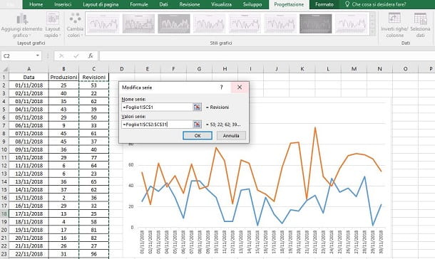
Once this is done, press the button OK, to view the data in the left section of the screen. Then click on the new dataset and verify that, on the right section, the values of column A are shown correctly. If not, press the button Modification that you find on the right and, in the box Axis label range, selects only the values in column A, not including the column label. Then press on OK twice consecutively: the first to confirm and the second to display the new data on the graph.
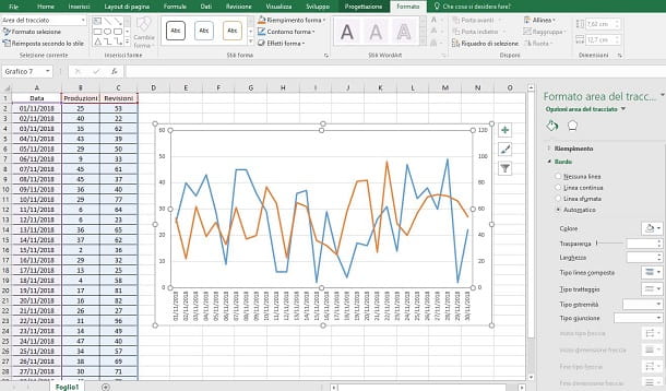
If the new dataset has a different scale than the previously added set, it might be useful to enable thesecondary Y axis. To do this, on the graph, double-click on the colored line corresponding to the data you want to move axis and, in the right sidebar that is shown to you, select the tab Series options, choosing the voice Secondary axis: by doing so, you will have shifted the Y values for that dataset from the left primary axis to the right secondary axis. This same procedure can be applied to multiple data sets in case you want to move them on the two different Y axes.
Customize a chart in Excel
Now that you have created your line chart in Excel, it may be appropriate to customize it, changing its colors and other elements, to better help interpret and identify the data. The customization options that I will show you in the next paragraphs are mostly contained in the tabs Planning e Format, which you find in the bar at the top, after selecting the graph.
If you want to change its layout, in the tab Planning, you can use the key Layout rapido. In the pane that is shown to you, you can see several predefined styles for displaying and distributing the elements of the chart. Via the button Change colors, you can instead choose to change the color sets according to some predefined templates. In the section Graphic styles you can also find line chart templates that you can use: you can enable styles with shading, with backgrounds and with different fonts and sizes.
If you don't want to rely on the predefined templates but want to make a creative customization, in the tab Format you can find all the tools you need: you can mark the outlines of the graph with different colors, using the menu Contour shape, or you can also add effects, such as shadows, using the button Shape effects. In the section Stili WordArt, you can change the color of the labels on the chart, its outline and you can also apply effects on them.
By then clicking on any element of the chart, using the right sidebar, you can customize each single element in detail, changing its color, font, stroke, effects, alignment and much more, using the tabs Fill and line, Effects, Dimensions: and properties e options.
In addition to what I indicated in the previous paragraphs, if you don't want to waste a lot of time designing and customizing a chart or spreadsheet for its presentation to colleagues and customers, you can use the predefined Excel templates. When you are on the new spreadsheet creation screen, you are presented with the option to choose one of the preset templates. Using the search bar at the top, type in the term graphic and, from the results that are shown to you, select the one that shows a line chart, suitable for your needs.
Make a line chart in Excel Online
If you need to use Excel, but the software is not installed on the computer you are using, you can orient your choice on the use of Excel Online, the web version of Microsoft's calculation program.
To use Excel Online all you need is a web browser, such as Google Chrome, Safari o Firefox, and a Microsoft account. Then reach the link I provided and type in the login credentials of your Microsoft account, so as to start using Excel Online.
On the main screen, click New blank workbook, useful for entering the dataset directly online. If so, you can first upload the Excel file to OneDrive, so you can open it directly with Excel Online, selecting the item Open from OneDrive, located at the bottom left of the spreadsheet creation screen.
The procedure for creating a line chart in Excel Online is similar to the one I told you about in the previous chapter. After selecting the data, you will find the button for creating the chart in the tab Inserisciby pressing the key Tiers and choosing Tiers o Lines with indicators, in the box that is shown to you.
Unlike the desktop version, Excel Online doesn't have many personalization and data organization tools. For example, you cannot arrange the data on two Y axes, thus having to uniform the data on a single scale. Also, there are no options for customizing colors and visual styles.
The only options available concern the activation and positioning of some elements of the chart, such as the title, the legend or the labels, for which you can find the appropriate buttons in the tab Graphic, after selecting the graph.
When you have finished your work, you can decide whether to export the file to a file XLSX (Fillet > Save with name > Download a copy) or share it with other users (Fillet > Share > Share with other users). In the latter case, you can decide whether to enter the Microsoft email addresses of the users with whom you want to share the file or generate a link accessible to all those to whom you send it.
Make a line chart on smartphones and tablets
Microsoft Excel can also be used in its version for mobile devices running Android, iOS and Windows 10 Mobile. The app is free, but requires a subscription to Office 365, in case it is installed on devices larger than 10.1 inches.
Additionally, some features, such as customizing PivotTable styles and layouts, multiple colors for shapes and formatting, adding elements to charts, and support for SmartArt, require a subscription to Office 365 with costs starting from 7 euros / month or 69 euros / year.
After starting the app Microsoft Excel, decide whether to open an Excel document present on the device memory (apri > This device) or from a file on OneDrive (apri > OneDrive Personal). If you need to create a new one, click onicon with a sheet that you find in the upper right corner and select Blank workbook.
After you have the table with the data set in front of you, highlight it by tapping on a cell and dragging theicon with a dot until you select all the cells to include in the chart (you must also highlight the column labels).
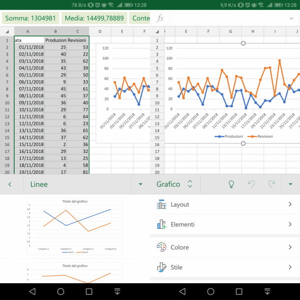
Once this is done, if you use a tablets, select the scheda Inserisci; if you use one smartphone, tap on the icon ▲ (Android) or ⋮ (iOS) located at the bottom right and tap the drop-down menu on the right, to select the item Inserisci. Then choose your options Graphic > Tiers, to instantly add a line chart to your spreadsheet.
The mobile version of Excel also has few customization features. Compared to the Web version, the Microsoft Excel app allows you to customize some aspects of the chart, such as the layout, colors and styles. All these features can be found by tapping on the graph, so as to view the card Graphic at the top (on a tablet) or at the bottom (on a smartphone).


![[Review] Samsung Powerbot VR7000: the robot vacuum cleaner from Star Wars](/images/posts/6bc44de38605b5c0fa12661febb1f8af-0.jpg)